《財務時間序列分析》線上附錄
R05:AAPL 的 ARMA 估計、診斷與預測
本附錄對應第 6–7 章,要完整走過一次實際的預測流程:只看 AAPL 的早期日對數報酬時,應如何選擇低階 ARMA 模型、檢查根與殘差,並在模型選定後評估未見期間?固定資料源自原課程 S&P 500 價格檔;每一列代表一個交易日,有效報酬樣本為 2019-01-03 至 2022-06-22,共 874 筆,單位是小數日對數報酬。資料建置方式見 data/DATA_SOURCES.md。
第 $t$ 日對數報酬要等當日調整收盤價可得後才能完整計算,所以本頁假設在訓練期最後一日收盤後形成預測。ARMA 模型描述的是 AAPL 報酬的條件平均動態;係數、診斷與預測誤差都沒有識別市場事件的因果效果,也不構成投資建議。
knitr::opts_chunk$set(
  echo = TRUE, message = FALSE, warning = FALSE,
  fig.width = 8, fig.height = 4.8,
  dev = "ragg_png", dpi = 144,
  dev.args = list(background = "white")
)

root_candidates <- c(".", "..")
is_root <- vapply(root_candidates, function(x) {
  file.exists(file.path(x, "main.tex"))
}, logical(1))
stopifnot(any(is_root))
project_root <- root_candidates[which(is_root)[1]]
project_path <- function(...) file.path(project_root, ...)

stopifnot(
  requireNamespace("ragg", quietly = TRUE),
  requireNamespace("systemfonts", quietly = TRUE)
)
cwtex_file <- project_path("assets", "fonts", "cwTeXQKai-Medium.ttf")
stopifnot(file.exists(cwtex_file))
if (!"cwTeX Online" %in% systemfonts::registry_fonts()$family) {
  systemfonts::register_font("cwTeX Online", cwtex_file)
}
plot_family <- "cwTeX Online"
固定資料與時間切分#
前 80% 報酬是訓練期,負責比較候選模型、計算 BIC 與估計所有參數;最後 20% 是一次性測試期,只負責回答選定模型在未見資料上的預測誤差。本例沒有另外設驗證期,因為調校工作都限於訓練期內的預先指定候選集合。測試期一旦被拿來改階數或改規格,就不再是未見測試資料。
aapl <- read.csv(project_path(
  "data", "processed", "aapl_adjusted_daily_2019_2022.csv"
))
aapl$date <- as.Date(aapl$date)
# 報酬的落後關係依日期而定,先排序再切分,不能隨機打散。
aapl <- aapl[order(aapl$date), ]
aapl <- aapl[is.finite(aapl$log_return), ]
row.names(aapl) <- NULL

stopifnot(
  !anyNA(aapl$date), !anyNA(aapl$log_return),
  all(diff(aapl$date) > 0)
)

y <- aapl$log_return
dates <- aapl$date
n <- length(y)
train_end <- floor(0.80 * n)
# 切點只由樣本長度決定,不參考後面的預測分數。
y_train <- y[seq_len(train_end)]
y_test <- y[(train_end + 1L):n]

split_table <- data.frame(
  區段 = c("訓練期", "測試期"),
  起日 = dates[c(1L, train_end + 1L)],
  迄日 = dates[c(train_end, n)],
  觀察值 = c(train_end, n - train_end),
  資料來源 = "原課程 S&P 500 價格檔的 AAPL 固定版本",
  單位 = "日對數報酬,小數",
  check.names = FALSE
)
knitr::kable(split_table)
| 區段 | 起日 | 迄日 | 觀察值 | 資料來源 | 單位 |
|---|---|---|---|---|---|
| 訓練期 | 2019-01-03 | 2021-10-11 | 699 | 原課程 S&P 500 價格檔的 AAPL 固定版本 | 日對數報酬,小數 |
| 測試期 | 2021-10-12 | 2022-06-22 | 175 | 原課程 S&P 500 價格檔的 AAPL 固定版本 | 日對數報酬,小數 |
表中訓練期為 2019-01-03 至 2021-10-11,共 699 筆;測試期為 2021-10-12 至 2022-06-22,共 175 筆。這裡評估的是「在 2021-10-11 收盤後一次形成,之後不重新估計」的多步預測。若希望每個交易日都加入新資訊並重新估計,應改用 R06 的擴展或滾動起點設計。
只在訓練期比較低階候選模型#
候選集合在讀取測試結果以前固定,只包含 $p,q\leq 2$ 的幾個低階模型。每個模型都用相同的 699 筆訓練資料與最大概似法估計,才可以公平比較 BIC。要注意,stats::arima() 對定態 ARMA 所報的 intercept 是序列平均數,而不是
$Y_t=c+\phi Y_{t-1}+a_t$ 中的 $c$。
candidate_orders <- list(
  ARMA00 = c(0, 0, 0),
  AR10 = c(1, 0, 0),
  MA01 = c(0, 0, 1),
  ARMA11 = c(1, 0, 1),
  AR20 = c(2, 0, 0),
  MA02 = c(0, 0, 2),
  ARMA21 = c(2, 0, 1),
  ARMA12 = c(1, 0, 2)
)

# 對每一個事前列出的階數,用同一估計法配適同一訓練期。
fits <- lapply(candidate_orders, function(ord) {
  arima(
    y_train,
    order = ord,
    include.mean = TRUE,
    method = "ML"
  )
})
stopifnot(all(vapply(fits, function(z) z$code == 0, logical(1))))

model_table <- data.frame(
  模型 = names(fits),
  p = vapply(candidate_orders, function(z) z[1], numeric(1)),
  q = vapply(candidate_orders, function(z) z[3], numeric(1)),
  對數概似 = vapply(fits, function(z) as.numeric(logLik(z)), numeric(1)),
  AIC = vapply(fits, AIC, numeric(1)),
  BIC = vapply(fits, BIC, numeric(1)),
  check.names = FALSE
)
model_table <- model_table[order(model_table$BIC), ]
row.names(model_table) <- NULL
knitr::kable(model_table, digits = 3)
| 模型 | p | q | 對數概似 | AIC | BIC |
|---|---|---|---|---|---|
| AR10 | 1 | 0 | 1692.238 | -3378.477 | -3364.828 |
| MA01 | 0 | 1 | 1691.150 | -3376.300 | -3362.651 |
| ARMA11 | 1 | 1 | 1692.452 | -3376.904 | -3358.705 |
| AR20 | 2 | 0 | 1692.444 | -3376.887 | -3358.689 |
| MA02 | 0 | 2 | 1692.226 | -3376.451 | -3358.253 |
| ARMA12 | 1 | 2 | 1692.452 | -3374.905 | -3352.156 |
| ARMA21 | 2 | 1 | 1692.452 | -3374.903 | -3352.155 |
| ARMA00 | 0 | 0 | 1678.042 | -3352.084 | -3342.985 |
selected_name <- model_table$模型[1]
selected_fit <- fits[[selected_name]]
selected_order <- candidate_orders[[selected_name]]
selected_name
## [1] "AR10"
表格由 BIC 小到大排列,這份訓練資料選出 AR(1)。BIC 只是在既定候選集合中的訓練期相對比較,不是測試期成績,也沒有保證候選集合包含真實資料生成過程。若所有候選模型的殘差都不理想,仍應降低結論強度或重新設計候選集合。
套件作法:用 auto.arima() 比較候選階數#
原課程的
slides/L04_ARMA/W1L4_R_template_for_estimating_ARMA.R
以 forecast::auto.arima() 選階、checkresiduals() 診斷,再以
forecast() 形成預測。
slides/L05_Forecasting_and_CV/W1L5_R_prediction_cv.R
另示範了不使用逐步搜尋的 AIC 選階。下列兩個套件版本都只讀訓練期:第一個把階數範圍與資訊準則限制成上一節的八種 $(p,d,q)$ 組合,但 auto.arima() 另會容許零平均規格,因此模型候選集合仍比手動版稍廣;第二個沿用原課程較自動的 AIC 搜尋。若要和手動版使用完全相同的候選集合,應逐一對 candidate_orders 呼叫 forecast::Arima(..., include.mean = TRUE, method = "ML"),再比較 BIC。auto.arima() 會代為估計與排序候選模型,卻不會替我們決定測試期何時開始、該採 AIC 或 BIC,或哪些階數具有實質上的合理性。
stopifnot(requireNamespace("forecast", quietly = TRUE))

# 階數範圍與手動版相同;auto.arima() 另會比較零平均規格。
fit_auto_matched <- forecast::auto.arima(
  y_train,
  d = 0,
  stationary = TRUE,
  seasonal = FALSE,
  max.p = 2,
  max.q = 2,
  max.order = 3,
  ic = "bic",
  stepwise = FALSE,
  approximation = FALSE,
  allowmean = TRUE
)

# 再沿用原課程 AIC 搜尋;階數仍只由訓練期決定。
fit_auto_course <- forecast::auto.arima(
  y_train,
  seasonal = FALSE,
  ic = "aic",
  stepwise = FALSE,
  approximation = FALSE
)

order_text <- function(fit) {
  order <- forecast::arimaorder(fit)[c("p", "d", "q")]
  sprintf("ARIMA(%d,%d,%d)", order["p"], order["d"], order["q"])
}

selection_comparison <- data.frame(
  方法 = c(
    "手動候選集/BIC",
    "forecast 同階數範圍/BIC",
    "forecast 原課程搜尋/AIC"
  ),
  選定模型 = c(
    sprintf(
      "ARIMA(%d,%d,%d)",
      selected_order[1], selected_order[2], selected_order[3]
    ),
    order_text(fit_auto_matched),
    order_text(fit_auto_course)
  ),
  對數概似 = c(
    as.numeric(logLik(selected_fit)),
    as.numeric(logLik(fit_auto_matched)),
    as.numeric(logLik(fit_auto_course))
  ),
  AIC = c(
    AIC(selected_fit), AIC(fit_auto_matched), AIC(fit_auto_course)
  ),
  BIC = c(
    BIC(selected_fit), BIC(fit_auto_matched), BIC(fit_auto_course)
  ),
  check.names = FALSE
)
knitr::kable(selection_comparison, digits = 3)
| 方法 | 選定模型 | 對數概似 | AIC | BIC |
|---|---|---|---|---|
| 手動候選集/BIC | ARIMA(1,0,0) | 1692.238 | -3378.477 | -3364.828 |
| forecast 同階數範圍/BIC | ARIMA(1,0,0) | 1692.238 | -3378.477 | -3364.828 |
| forecast 原課程搜尋/AIC | ARIMA(2,0,3) | 1708.172 | -3402.344 | -3370.497 |
同階數範圍搜尋與手動表若選到相同結果,只能說兩者在這份資料上的相對勝者一致;由於前者另容許零平均,不能據此宣稱候選集合完全相同。若兩者結果不同,應先檢查平均數規格;若要逐模型核對,則應使用前述 forecast::Arima() 寫法固定每個階數與 include.mean = TRUE。原課程 AIC 版本的搜尋範圍與懲罰也不同,選到另一個階數時,差異來自研究設定而非套件失靈。報告「自動選階」結果時,仍要一併寫清楚資訊準則、搜尋範圍、平均數規格與訓練期間。
係數、定態根與可逆根#
選定階數後,先讀係數的方向與不確定性,再檢查 AR 與 MA 多項式的根。係數表的每一列是一個參數,估計值 與 標準誤 使用日對數報酬的小數尺度;根表則列出複數根的實部、虛部與模。
coefficient_table <- data.frame(
  參數 = names(coef(selected_fit)),
  估計值 = as.numeric(coef(selected_fit)),
  標準誤 = sqrt(diag(selected_fit$var.coef)),
  check.names = FALSE
)
knitr::kable(coefficient_table, digits = 6)
| 參數 | 估計值 | 標準誤 | |
|---|---|---|---|
| ar1 | ar1 | -0.202870 | 0.037686 |
| intercept | intercept | 0.001906 | 0.000677 |
extract_roots <- function(fit) {
  b <- coef(fit)
  ar_coef <- b[grep("^ar[0-9]+$", names(b))]
  ma_coef <- b[grep("^ma[0-9]+$", names(b))]

  # AR 與 MA 多項式的符號不同,分開建立可避免根的方向寫反。
  ar_roots <- if (length(ar_coef)) {
    polyroot(c(1, -ar_coef))
  } else {
    complex()
  }
  ma_roots <- if (length(ma_coef)) {
    polyroot(c(1, ma_coef))
  } else {
    complex()
  }

  rbind(
    if (length(ar_roots)) data.frame(
      部分 = "AR", 實部 = Re(ar_roots), 虛部 = Im(ar_roots), 模 = Mod(ar_roots)
    ),
    if (length(ma_roots)) data.frame(
      部分 = "MA", 實部 = Re(ma_roots), 虛部 = Im(ma_roots), 模 = Mod(ma_roots)
    )
  )
}

root_table <- extract_roots(selected_fit)
if (nrow(root_table)) {
  knitr::kable(root_table, digits = 5)
  stopifnot(all(root_table$模 > 1))
} else {
  cat("所選模型沒有 AR 或 MA 根需要檢查。\n")
}
所選 AR(1) 的 AR 係數約為 -0.2029,標準誤約為 0.0377;intercept 約為 0.001906,這裡代表訓練期估計的序列平均數。負的 AR 係數表示報酬偏離平均數後,下一日的條件平均有短期反向調整,但它只是樣本內的縮減式動態,不能解讀成可交易策略或因果反應。
AR 根在單位圓外時,估計模型具有因果定態表示;若模型含 MA 項,MA 根在單位圓外則表示可逆。根通過條件是採用模型的必要檢查,還不是充分診斷;根接近 1 時,有限樣本推論與遠期預測仍可能不穩定。
訓練期殘差診斷#
資訊準則選出相對勝者後,要問的是它是否已把可預測的平均動態留在殘差之外。第一列 Ljung–Box 檢查殘差前 20 階的線性相依,並扣除已估的 AR 與 MA 參數自由度;第二列檢查平方殘差,尋找尚未處理的波動群聚。
selected_residual <- as.numeric(residuals(selected_fit))
selected_residual <- selected_residual[is.finite(selected_residual)]
p_plus_q <- selected_order[1] + selected_order[3]

# 平均方程的檢定扣除 p+q;平方殘差列用來診斷波動,不沿用同一 fitdf。
q_mean <- Box.test(
  selected_residual, lag = 20, type = "Ljung-Box",
  fitdf = p_plus_q
)
q_square <- Box.test(
  selected_residual^2, lag = 20, type = "Ljung-Box"
)

diagnostic_table <- data.frame(
  檢查對象 = c("殘差", "平方殘差"),
  Q20 = c(unname(q_mean$statistic), unname(q_square$statistic)),
  自由度 = c(unname(q_mean$parameter), unname(q_square$parameter)),
  p值 = c(q_mean$p.value, q_square$p.value),
  check.names = FALSE
)
knitr::kable(diagnostic_table, digits = 6)
| 檢查對象 | Q20 | 自由度 | p值 |
|---|---|---|---|
| 殘差 | 54.18846 | 19 | 3.1e-05 |
| 平方殘差 | 355.02037 | 20 | 0.0e+00 |
本次 AR(1) 殘差的 Ljung–Box $p$ 值約為 $3.1\times10^{-5}$,平方殘差的 $p$ 值更接近零。這是明確的診斷警訊:BIC 所選模型只是候選集合內的相對勝者,並未清除全部平均與波動相依。平均殘差的結果提示可以檢查其他低階規格;平方殘差則提示把 ARCH/GARCH 類模型納入後續分析。
matched_order <- forecast::arimaorder(fit_auto_matched)[c("p", "d", "q")]
matched_residual <- as.numeric(residuals(fit_auto_matched))
matched_residual <- matched_residual[is.finite(matched_residual)]
matched_df <- matched_order["p"] + matched_order["q"]

matched_q_mean <- Box.test(
  matched_residual,
  lag = 20,
  type = "Ljung-Box",
  fitdf = matched_df
)
matched_q_square <- Box.test(
  matched_residual^2,
  lag = 20,
  type = "Ljung-Box"
)

diagnostic_comparison <- data.frame(
  方法 = rep(c("手動候選集", "forecast 同階數範圍搜尋"), each = 2),
  檢查對象 = rep(c("殘差", "平方殘差"), 2),
  Q20 = c(
    unname(q_mean$statistic), unname(q_square$statistic),
    unname(matched_q_mean$statistic),
    unname(matched_q_square$statistic)
  ),
  p值 = c(
    q_mean$p.value, q_square$p.value,
    matched_q_mean$p.value, matched_q_square$p.value
  ),
  check.names = FALSE
)
knitr::kable(diagnostic_comparison, digits = 7)
| 方法 | 檢查對象 | Q20 | p值 |
|---|---|---|---|
| 手動候選集 | 殘差 | 54.18846 | 3.09e-05 |
| 手動候選集 | 平方殘差 | 355.02037 | 0.00e+00 |
| forecast 同階數範圍搜尋 | 殘差 | 54.19123 | 3.09e-05 |
| forecast 同階數範圍搜尋 | 平方殘差 | 355.02619 | 0.00e+00 |
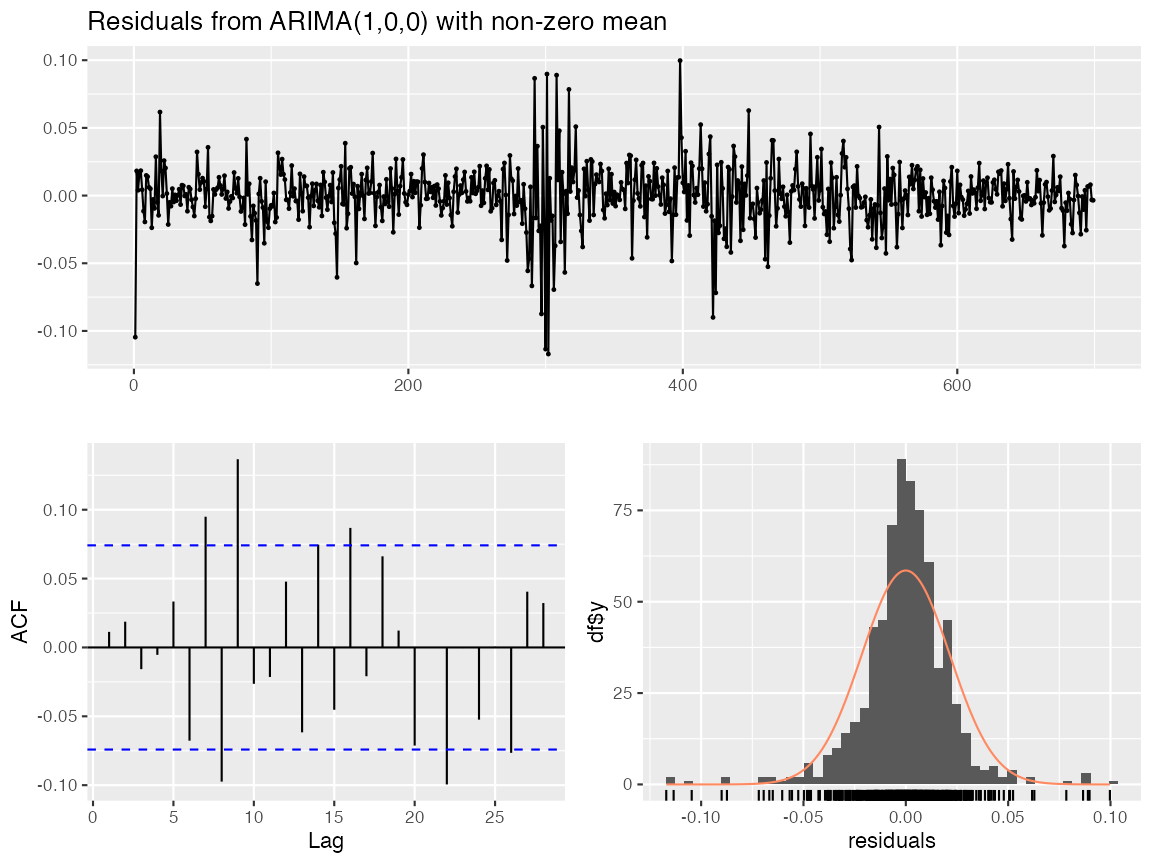
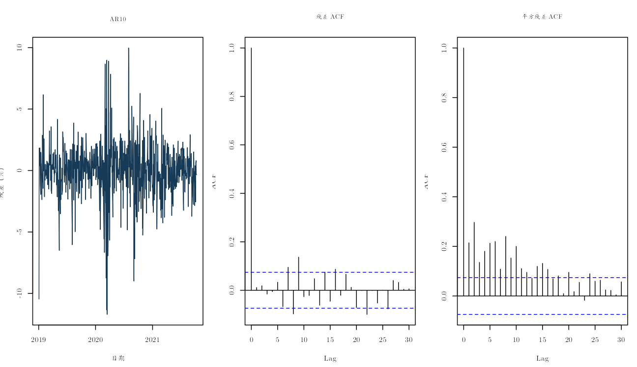
# 原課程使用的一行診斷,同時呈現殘差路徑、ACF 與聯合檢定。
forecast::checkresiduals(fit_auto_matched, lag = 20)
##
##  Ljung-Box test
##
## data:  Residuals from ARIMA(1,0,0) with non-zero mean
## Q* = 54.191, df = 19, p-value = 3.089e-05
##
## Model df: 1.   Total lags used: 20
若同階數範圍搜尋與手動程式不只選到相同階數,也採用相同的平均數規格,上表的兩組診斷才應幾乎重合。小數點差異可能來自初始化與數值容差;若模型階數、平均數規格或自由度不同,就要先統一這些設定、估計法與 fitdf,才能把 Ljung–Box 數值放在同一基準上比較。checkresiduals() 替我們排好圖與檢定,仍需由讀者根據殘差或平方殘差的警訊決定下一步。
old_par <- par(
  mfrow = c(1, 3), mar = c(4.5, 3.5, 4, 1),
  family = plot_family, cex.main = 0.88
)
plot(
  dates[seq_along(selected_residual)], 100 * selected_residual,
  type = "l", col = "#173B57",
  xlab = "日期", ylab = "殘差(%)", main = selected_name
)
acf(selected_residual, lag.max = 30, main = "殘差 ACF")
acf(selected_residual^2, lag.max = 30, main = "平方殘差 ACF")
par(old_par)
圖形補上檢定數字沒有呈現的資訊:殘差時間圖可以看出警訊集中在哪些日期,兩張 ACF 則顯示相依落在何種期距。由於殘差仍有線性相依,所選低階平均數模型只能視為候選集合中的相對勝者;平方殘差的明顯相依則是第 11–12 章 ARCH/GARCH 模型的直接動機。
選定模型後的一次多步預測#
現在才讓模型面對保留的 175 筆測試資料。predict() 在訓練期末使用已估的 AR(1) 係數,一次產生整段多步預測;測試期內即使已經觀察到新的實際報酬,也不把它加入模型。這個設計回答「若在 2021-10-11 只估計一次,遠期預測會如何」,與每日更新的一步預測是不同問題。
h <- length(y_test)
# 模型、參數與預測起點都在讀取測試答案前選定。
forecast_object <- predict(selected_fit, n.ahead = h)

forecast_table <- data.frame(
  日期 = dates[(train_end + 1L):n],
  實際值 = y_test,
  ARMA預測 = as.numeric(forecast_object$pred),
  預測標準誤 = as.numeric(forecast_object$se),
  check.names = FALSE
)
forecast_table$下界95 <- forecast_table$ARMA預測 -
  1.96 * forecast_table$預測標準誤
forecast_table$上界95 <- forecast_table$ARMA預測 +
  1.96 * forecast_table$預測標準誤
forecast_table$ARMA誤差 <- forecast_table$實際值 -
  forecast_table$ARMA預測

knitr::kable(head(forecast_table, 8), digits = 6)
| 日期 | 實際值 | ARMA預測 | 預測標準誤 | 下界95 | 上界95 | ARMA誤差 |
|---|---|---|---|---|---|---|
| 2021-10-12 | -0.009145 | 0.002420 | 0.021496 | -0.039711 | 0.044552 | -0.011565 |
| 2021-10-13 | -0.004249 | 0.001802 | 0.021933 | -0.041188 | 0.044791 | -0.006051 |
| 2021-10-14 | 0.020024 | 0.001927 | 0.021951 | -0.041097 | 0.044952 | 0.018097 |
| 2021-10-15 | 0.007485 | 0.001902 | 0.021952 | -0.041124 | 0.044928 | 0.005583 |
| 2021-10-18 | 0.011737 | 0.001907 | 0.021952 | -0.041119 | 0.044933 | 0.009830 |
| 2021-10-19 | 0.014968 | 0.001906 | 0.021952 | -0.041120 | 0.044932 | 0.013062 |
| 2021-10-20 | 0.003356 | 0.001906 | 0.021952 | -0.041120 | 0.044932 | 0.001450 |
| 2021-10-21 | 0.001473 | 0.001906 | 0.021952 | -0.041120 | 0.044932 | -0.000433 |
表中每一列是一個測試交易日:ARMA預測 是訓練期末可形成的條件平均預測,預測標準誤 隨期距反映未來創新累積,實際值 只在事後計分時使用。任何一列的實際值都沒有回流到後面日期的預測。
score_row <- function(actual, forecast, label) {
  error <- actual - forecast
  data.frame(
    模型 = label,
    RMSE = sqrt(mean(error^2)),
    MAE = mean(abs(error)),
    平均誤差 = mean(error),
    check.names = FALSE
  )
}

score_table <- rbind(
  score_row(y_test, forecast_table$ARMA預測, selected_name),
  score_row(y_test, rep(0, h), "零報酬"),
  score_row(y_test, rep(mean(y_train), h), "訓練期平均數")
)
score_table$常態區間涵蓋率 <- c(
  mean(
    y_test >= forecast_table$下界95 &
      y_test <= forecast_table$上界95
  ),
  NA_real_, NA_real_
)
knitr::kable(score_table, digits = 6)
| 模型 | RMSE | MAE | 平均誤差 | 常態區間涵蓋率 |
|---|---|---|---|---|
| AR10 | 0.020809 | 0.016036 | -0.002191 | 0.977143 |
| 零報酬 | 0.020694 | 0.015951 | -0.000283 | NA |
| 訓練期平均數 | 0.020805 | 0.016031 | -0.002162 | NA |
RMSE 對較大的預測錯誤給予更高權重,MAE 則以絕對誤差計分,平均誤差用來觀察預測是否整體偏高或偏低。在這 175 筆固定測試資料中,零報酬基準的 RMSE 與 MAE 都略低於訓練期 BIC 所選的 AR(1)。這個結果很有教學價值:樣本內資訊準則較佳,不保證樣本外預測勝過簡單基準。既然測試答案已經看過,就不應再為了追上零報酬基準而回頭改階數。
套件作法:用 forecast() 形成預測並以 accuracy() 計分#
下列程式對前面兩個 auto.arima() 模型執行原課程採用的
forecast() 與 accuracy() 工作流程。forecast() 會整理點預測與區間,accuracy() 會依實際值計算常用誤差指標;兩者都不會替我們維持樣本外紀律。因此,兩個模型的階數仍在訓練期選定,測試期只用來計分。
course_forecast_matched <- forecast::forecast(
  fit_auto_matched,
  h = h,
  level = 95
)
course_forecast_aic <- forecast::forecast(
  fit_auto_course,
  h = h,
  level = 95
)

accuracy_row <- function(object, actual, label) {
  # accuracy() 可能同時回報訓練與測試列;此處明確取最後一列測試結果。
  package_accuracy <- forecast::accuracy(object, actual)
  test_accuracy <- package_accuracy[nrow(package_accuracy), , drop = FALSE]
  data.frame(
    模型 = label,
    RMSE = unname(test_accuracy[1, "RMSE"]),
    MAE = unname(test_accuracy[1, "MAE"]),
    平均誤差 = unname(test_accuracy[1, "ME"]),
    常態區間涵蓋率 = mean(
      actual >= as.numeric(object$lower[, 1]) &
        actual <= as.numeric(object$upper[, 1])
    ),
    check.names = FALSE
  )
}

manual_accuracy <- score_row(
  y_test,
  forecast_table$ARMA預測,
  paste0("手動候選:", selected_name)
)
manual_accuracy$常態區間涵蓋率 <- mean(
  y_test >= forecast_table$下界95 &
    y_test <= forecast_table$上界95
)

zero_accuracy <- score_row(y_test, rep(0, h), "零報酬")
zero_accuracy$常態區間涵蓋率 <- NA_real_

package_forecast_comparison <- rbind(
  manual_accuracy,
  accuracy_row(
    course_forecast_matched,
    y_test,
    paste0("forecast 同階數範圍BIC:", order_text(fit_auto_matched))
  ),
  accuracy_row(
    course_forecast_aic,
    y_test,
    paste0("forecast 原課程AIC:", order_text(fit_auto_course))
  ),
  zero_accuracy
)
row.names(package_forecast_comparison) <- NULL
knitr::kable(package_forecast_comparison, digits = 7)
| 模型 | RMSE | MAE | 平均誤差 | 常態區間涵蓋率 |
|---|---|---|---|---|
| 手動候選:AR10 | 0.0208091 | 0.0160361 | -0.0021910 | 0.9771429 |
| forecast 同階數範圍BIC:ARIMA(1,0,0) | 0.0208091 | 0.0160361 | -0.0021907 | 0.9771429 |
| forecast 原課程AIC:ARIMA(2,0,3) | 0.0208093 | 0.0160548 | -0.0022301 | 0.9771429 |
| 零報酬 | 0.0206943 | 0.0159514 | -0.0002826 | NA |
若手動 BIC 與同階數範圍的 auto.arima() 不只選到同一階數,也採用相同平均數規格,兩者點預測與評分才應幾乎相同。只看階數相同,還不足以宣稱兩套程式估的是同一個模型。原課程 AIC 版本可能選到不同階數,因而產生不同預測。比較表要連同模型標籤一起讀,不能只挑 RMSE 最小的一列,事後把它說成事前選定的模型。
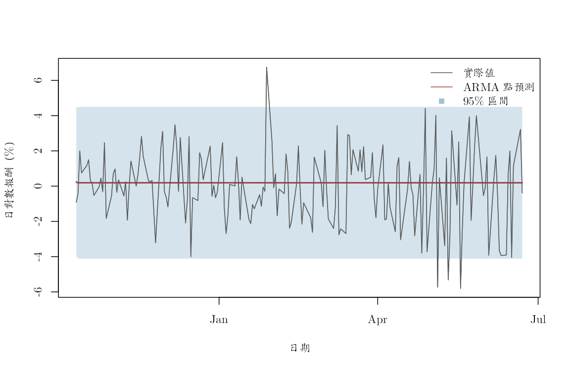
old_par <- par(family = plot_family)
plot(
  forecast_table$日期, 100 * forecast_table$實際值,
  type = "l", col = "gray35",
  xlab = "日期", ylab = "日對數報酬(%)"
)
polygon(
  c(forecast_table$日期, rev(forecast_table$日期)),
  100 * c(forecast_table$下界95, rev(forecast_table$上界95)),
  border = NA, col = adjustcolor("#9FC2D4", alpha.f = 0.45)
)
lines(
  forecast_table$日期, 100 * forecast_table$ARMA預測,
  col = "#A34045", lwd = 2
)
lines(
  forecast_table$日期, 100 * forecast_table$實際值,
  col = "gray35"
)
legend(
  "topright", c("實際值", "ARMA 點預測", "95% 區間"),
  col = c("gray35", "#A34045", "#9FC2D4"),
  lty = c(1, 1, NA), pch = c(NA, NA, 15), bty = "n"
)
par(old_par)
圖中帶狀區域是以所選 ARMA 模型與常態近似形成的 95% 區間,主要反映未來創新的不確定性。它沒有完整納入參數估計、階數選擇、厚尾與條件異質變異造成的不確定性。表中的固定測試期涵蓋率只能描述這 175 筆觀察值;若涵蓋不足,下一步應檢查創新分配與波動模型,而不是任意加寬區間到看起來理想。
用已知真值確認符號與估計流程#
最後另生成一條 5,000 期的 ARMA(1,1) 模擬序列。因為 AR 與 MA 真值已知,我們可以確認 arima() 的係數符號與名稱是否和課文一致。這條模擬序列只檢查程式流程,不參與 AAPL 的模型選擇、預測評分或實證結論。
set.seed(20260721)
truth <- c(ar1 = 0.55, ma1 = -0.35)
simulated_check <- as.numeric(arima.sim(
  model = list(ar = truth["ar1"], ma = truth["ma1"]),
  n = 5000, sd = 0.01
))
fit_check <- arima(
  simulated_check, order = c(1, 0, 1),
  include.mean = TRUE, method = "ML"
)
check_table <- data.frame(
  參數 = names(truth),
  真值 = truth,
  估計值 = coef(fit_check)[names(truth)],
  check.names = FALSE
)
knitr::kable(check_table, digits = 4)
| 參數 | 真值 | 估計值 | |
|---|---|---|---|
| ar1 | ar1 | 0.55 | 0.5673 |
| ma1 | ma1 | -0.35 | -0.3769 |
stopifnot(max(abs(check_table$估計值 - check_table$真值)) < 0.10)
兩個估計值與真值的差距都應小於事前設定的 0.10 容許範圍。若沒有通過,應先檢查 MA 符號慣例、係數名稱與模擬長度,而不能據此修改 AAPL 的實證模型。
如何延伸這次結果#
這份 AAPL 固定樣本顯示,訓練期 BIC 在既定候選集合中選出 AR(1),但殘差與平方殘差仍有明顯相依,而且一次形成的多步預測沒有勝過零報酬基準。可以得到的結論是:這個低階條件平均模型尚不足以完整描述資料,也沒有展現穩健的樣本外優勢;我們還不能把負 AR 係數解讀成可交易規律。
下一步可在新的訓練/驗證設計中納入其他平均規格與 ARCH/GARCH 波動模型,再保留另一段未見期間評估。報告時應保存固定資料版本、訓練截止日、候選集合、估計方法、截距參數化、資訊準則、根、殘差診斷、預測期距與區間假設。若看過這 175 筆測試結果後再換模型,這段期間就只能當作驗證資料;新的主張需要另一段真正未見的測試期。