《財務時間序列分析》線上附錄
R15:加州學校資料的雙重選擇與 DML 式殘差化
本附錄要回答一個高維迴歸問題:控制 93 個學校、學區與郵遞區號背景變數後,師生比與五年級測驗分數之間還剩下多少線性關聯?資料是加州學校的橫斷面,每一列代表一所學校。應變數 testscore 是英文/語文與數學分數合計,單位為測驗分數點;焦點解釋變數 str_s 是每位全職當量教師所對應的學生數。我們依序使用雙重選擇(double selection)與交叉配適的雙重/去偏機器學習(double/debiased machine learning, DML)式殘差化來估計這項條件關聯。本頁借用 DML 的交叉配適與正交評分想法,但不把它誤寫成已具備因果識別的完整 DML 研究。
這裡的目標參數是指定控制字典下的部分線性投影係數。資料沒有可核實的觀察年度或處置先後,也沒有驗證無未觀察混淆、重疊、穩定單位處置值及控制變數皆在處置前決定。因此主結果應讀成師生比與測驗分數的條件關聯;交叉配適與正交評分函數改善高維估計程序,並不自行建立班級規模的因果識別。
這不是樣本外預測比較,所以不另留最終測試樣本。3,932 所學校共同構成目標樣本;雙重選擇用學區分組的交叉驗證挑選懲罰參數,DML 式殘差化則以外層折產生交叉配適殘差、再在每個外層訓練樣本內用內層折調校。外層保留折的角色是避免同一筆觀察同時訓練干擾函數與計算自身分數,不是看完後挑選模型的測試樣本。
knitr::opts_chunk$set(
  echo = TRUE, message = FALSE, warning = FALSE,
  fig.width = 8, fig.height = 5,
  dev = "ragg_png", dpi = 144,
  dev.args = list(background = "white")
)
stopifnot(getRversion() >= "4.3.0")
if (!requireNamespace("glmnet", quietly = TRUE)) {
  stop("本附錄需要 glmnet;請先在合法可重現環境中安裝。")
}
set.seed(1515)

root_candidates <- c(".", "..")
is_root <- vapply(root_candidates, function(x) {
  file.exists(file.path(x, "main.tex"))
}, logical(1))
stopifnot(any(is_root))
project_root <- root_candidates[which(is_root)[1]]
project_path <- function(...) file.path(project_root, ...)

stopifnot(
  requireNamespace("ragg", quietly = TRUE),
  requireNamespace("systemfonts", quietly = TRUE)
)
cwtex_file <- project_path("assets", "fonts", "cwTeXQKai-Medium.ttf")
stopifnot(file.exists(cwtex_file))
if (!"cwTeX Online" %in% systemfonts::registry_fonts()$family) {
  systemfonts::register_font("cwTeX Online", cwtex_file)
}
plot_family <- "cwTeX Online"
一列資料代表什麼?#
資料來源是原課程的 Stock and Watson《Introduction to Econometrics》第四版 California school test-score 資料與變數表。每列是一所學校,schoolcode 在檔內唯一;樣本有 3,932 所學校。固定檔沒有可供本附錄核實的觀察年度欄位,因此不自行推定年份,也不把橫斷面差異寫成時間變化。
本頁直接讀取專案內保存的 california_schools.csv 整理後快照。若要由教材來源重新建檔,仍須記錄教材版次、資料檔版本、下載日與變數表。
locate_project_file <- function(relative_path) {
  candidates <- c(
    relative_path,
    file.path("..", relative_path),
    file.path("../..", relative_path)
  )
  hit <- candidates[file.exists(candidates)]
  if (length(hit) == 0L) stop("找不到專案檔案:", relative_path)
  normalizePath(hit[1], mustWork = TRUE)
}

school_file <- locate_project_file("data/processed/california_schools.csv")
manifest_file <- locate_project_file("data/processed/manifest.csv")
school <- read.csv(school_file, stringsAsFactors = FALSE, check.names = FALSE)
manifest <- read.csv(manifest_file, stringsAsFactors = FALSE)

manifest_key <- "data/processed/california_schools.csv"
manifest_row <- manifest[manifest$file == manifest_key, , drop = FALSE]
actual_md5 <- unname(tools::md5sum(school_file))

stopifnot(
  nrow(school) == 3932L,
  ncol(school) == 110L,
  nrow(manifest_row) == 1L,
  identical(actual_md5, manifest_row$md5),
  !anyDuplicated(school$schoolcode),
  !anyNA(school[c("testscore", "str_s", "districtcode")])
)

data.frame(
  學校數 = nrow(school),
  學區數 = length(unique(school$districtcode)),
  不重複學校代碼數 = length(unique(school$schoolcode)),
  應變數單位 = "測驗分數點",
  焦點解釋變數單位 = "每位全職當量教師所對應的學生數",
  觀察年度 = "固定檔未記錄",
  MD5 = actual_md5,
  check.names = FALSE
)
##   學校數 學區數 不重複學校代碼數 應變數單位               焦點解釋變數單位
## 1   3932    464             3932 測驗分數點 每位全職當量教師所對應的學生數
##       觀察年度                              MD5
## 1 固定檔未記錄 28b3dff5db50448608925cad32feb18a
summary(school[c("testscore", "str_s")])
##    testscore         str_s
##  Min.   :575.7   Min.   :10.66
##  1st Qu.:706.5   1st Qu.:21.08
##  Median :747.5   Median :23.81
##  Mean   :752.1   Mean   :23.64
##  3rd Qu.:792.4   3rd Qu.:26.25
##  Max.   :983.1   Max.   :33.71
輸出核對三件事:3,932 所學校分布在 464 個學區、學校編號沒有重複,而且 testscore、str_s 與學區編號皆無缺值。摘要表也保留兩個原始單位;後面 str_s 的係數一律解讀為「每位教師所對應學生數增加 1 人時,測驗分數相差多少點」。
建立高維背景控制字典#
控制字典先排除英文與數學分項分數,因為兩者機械地組成 testscore;名稱、行政區與學校編號、郵遞區號、師生比本身、學區師生比,以及直接構成學校師生比的學生數與全職當量教師數也不進入。留下的數值欄涵蓋餐費資格、英語學習、族群組成、教師經驗、學區財務與郵遞區號人口背景。
這 93 欄構成一組明示的條件調整集合。其中仍可能有與師生比同步決定或在其後形成的變數,所以本頁用它來比較條件關聯,不把它當成已由研究設計證成的因果混淆集合。
excluded <- c(
  "countyname", "districtname", "schoolname",
  "countycode", "districtcode", "schoolcode", "charternumber", "zipcode",
  "elarts_score", "math_score", "testscore",
  "str_s", "str_d", "te_fte_s", "te_fte_d",
  "enrollment_star_s", "enrollment_s"
)

control_names <- setdiff(names(school), excluded)
control_names <- control_names[vapply(
  school[control_names], is.numeric, logical(1)
)]
X_raw <- as.matrix(school[, control_names, drop = FALSE])
storage.mode(X_raw) <- "double"

nonconstant <- apply(X_raw, 2, sd) > 1e-10
X_raw <- X_raw[, nonconstant, drop = FALSE]
control_names <- colnames(X_raw)

Y <- school$testscore
D <- school$str_s
cluster <- school$districtcode

stopifnot(
  !anyNA(X_raw), all(is.finite(X_raw)),
  ncol(X_raw) == 93L,
  length(Y) == nrow(X_raw)
)

# 保留控制變數的原始數值;glmnet 會在每一個實際訓練樣本內重新標準化。
# 因此,外層保留學區的分布不會參與干擾函數學習器的前處理。
X <- X_raw
data.frame(
  observations = nrow(X),
  controls = ncol(X),
  outcome = "testscore",
  focal_exposure = "str_s",
  clustering_level = "districtcode"
)
##   observations controls   outcome focal_exposure clustering_level
## 1         3932       93 testscore          str_s     districtcode
套件作法:用 cv.glmnet() 選擇與預測背景變數#
這段沿用原課程以 LASSO 處理高維控制的工作流程。cv.glmnet() 代做係數路徑、訓練樣本內的標準化與給定折下的交叉驗證;分析者仍要決定哪些欄可進控制字典、折如何形成,以及採用 lambda.1se 或 lambda.min。本頁把同一學區的學校放在同一折,讓學區共同環境不會同時出現在訓練資料與保留資料中。雙重選擇採較簡約的 lambda.1se;DML 式干擾函數配適採 lambda.min,而且每個外層訓練樣本都重新做一次內層調校。
make_group_folds <- function(group, K, seed) {
  set.seed(seed)
  groups <- sample(unique(group))
  mapping <- setNames(rep(seq_len(K), length.out = length(groups)), groups)
  unname(mapping[as.character(group)])
}

fit_lasso_cv <- function(X, y, fold_id, s = "lambda.1se") {
  cv <- glmnet::cv.glmnet(
    x = X, y = y,
    alpha = 1, standardize = TRUE, intercept = TRUE,
    foldid = fold_id
  )
  beta <- as.matrix(stats::coef(cv, s = s))[-1, 1]
  names(beta) <- colnames(X)
  list(
    fit = cv,
    beta = beta,
    selected = which(abs(beta) > 1e-10),
    lambda = if (s == "lambda.min") cv$lambda.min else cv$lambda.1se
  )
}
雙重選擇:兩條路徑都可能找到重要控制#
若某個控制變數主要預測師生比、卻只弱度預測測驗分數,只沿應變數路徑選變數便可能漏掉它。雙重選擇先分別用 LASSO 找出與 testscore、str_s 有關的控制,再取兩者聯集,重估 testscore 對 str_s 與所選控制的線性投影。標準誤按學區叢聚,用來處理同一學區學校的相關性;但一般的叢聚穩健三明治公式不會自動處理所有變數選擇不確定性。要把它當成具有名目涵蓋率的高維推論,還需要近似稀疏性、適當懲罰率、設計條件與足夠群組數等假設。因此本頁把它標成描述性的後選擇 OLS 標準誤,並把後面的交叉配適正交分數作為較主要的高維估計結果。
selection_fold <- make_group_folds(cluster, K = 10L, seed = 1515)
fit_y <- fit_lasso_cv(X, Y, selection_fold, s = "lambda.1se")
fit_d <- fit_lasso_cv(X, D, selection_fold, s = "lambda.1se")
selected_union <- sort(unique(c(fit_y$selected, fit_d$selected)))

data.frame(
  path = c("Y on X", "D on X", "union"),
  selected_controls = c(
    length(fit_y$selected),
    length(fit_d$selected),
    length(selected_union)
  ),
  lambda = c(fit_y$lambda, fit_d$lambda, NA_real_)
)
##     path selected_controls    lambda
## 1 Y on X                19 2.3108544
## 2 D on X                15 0.1443038
## 3  union                28        NA
fit_conditional_projection <- function(selected, Y, D, X, cluster) {
  X_selected <- X[, selected, drop = FALSE]
  if (length(selected) > 0L) {
    # 後選擇 OLS 使用全樣本估計;在這裡標準化只改善數值條件,
    # 不改變焦點變數 str_s 的原始單位。
    X_selected <- scale(X_selected)
  }
  Z <- cbind(Intercept = 1, str_s = D, X_selected)

  # 移除精確或近精確線性相依欄,避免反矩陣不穩;焦點 D 固定保留。
  qrz <- qr(Z, tol = 1e-5, LAPACK = FALSE)
  keep <- sort(qrz$pivot[seq_len(qrz$rank)])
  if (!("str_s" %in% colnames(Z)[keep])) stop("焦點變數在降秩時被移除。")
  Z_use <- Z[, keep, drop = FALSE]

  fit <- lm.fit(Z_use, Y)
  residual <- fit$residuals
  # 先在學區內加總分數,再形成 sandwich 估計量的中間矩陣,保留學區內相依。
  cluster_score <- rowsum(Z_use * residual, cluster, reorder = FALSE)
  bread <- solve(crossprod(Z_use))
  G <- nrow(cluster_score)
  n <- nrow(Z_use)
  k <- ncol(Z_use)
  correction <- (G / (G - 1)) * ((n - 1) / (n - k))
  V_cluster <- correction * bread %*%
    crossprod(cluster_score) %*% bread

  j <- match("str_s", colnames(Z_use))
  c(
    estimate = fit$coefficients[j],
    post_selection_district_cluster_se_descriptive =
      sqrt(V_cluster[j, j]),
    selected_controls = length(selected),
    regression_rank = ncol(Z_use)
  )
}

naive_projection <- fit_conditional_projection(
  integer(0), Y, D, X, cluster
)
double_selection <- fit_conditional_projection(
  selected_union, Y, D, X, cluster
)

rbind(
  unadjusted_linear_projection = naive_projection,
  double_selection_projection = double_selection
)
##                              estimate.str_s
## unadjusted_linear_projection       1.904961
## double_selection_projection        0.254675
##                              post_selection_district_cluster_se_descriptive
## unadjusted_linear_projection                                      0.5591443
## double_selection_projection                                       0.2783569
##                              selected_controls regression_rank
## unadjusted_linear_projection                 0               2
## double_selection_projection                 28              30
未調整投影斜率約為 1.90;加入雙重選擇得到的 28 個控制後,斜率降到約 0.25。變化幅度顯示學校背景組成與師生比、測驗分數都有密切關係。調整後估計值相對其描述性後選擇學區叢聚標準誤並不大,適合保守地描述為接近零的條件線性關聯;它仍不是師生比的因果效果,也不能只因表中附有叢聚標準誤就視為已處理全部選擇不確定性。
學區群組交叉配適的 DML 式殘差化#
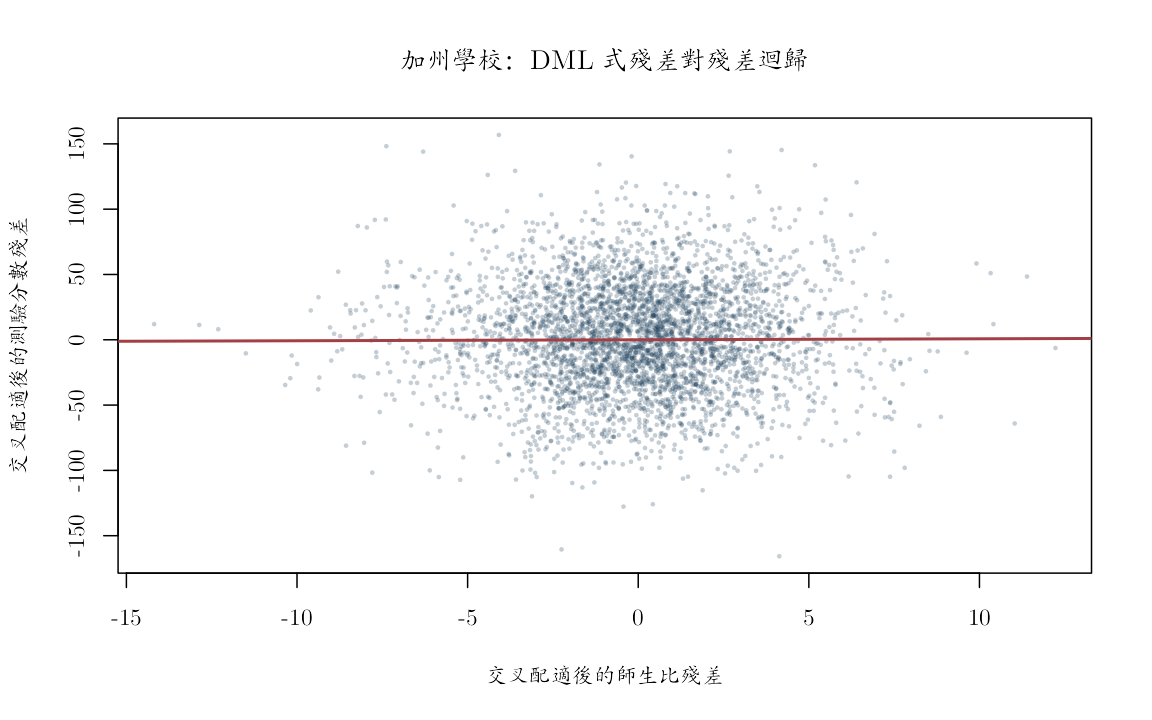
令 \(\ell(X)=E[Y\mid X]\)、\(m(X)=E[D\mid X]\)。每個外層保留學區只接受其他學區訓練出的預測,因此同一所學校不會同時參與干擾函數配適與自身殘差計算。接著以
\[ \widehat\theta= \frac{\sum_i \widehat v_i\widehat u_i} {\sum_i \widehat v_i^2},\qquad \widehat u_i=Y_i-\widehat\ell(X_i),\quad \widehat v_i=D_i-\widehat m(X_i) \]
估計殘差化係數。分子比較「背景變數無法預測的師生比」與「背景變數無法預測的測驗分數」是否共同變動;分母則衡量控制背景後還剩多少師生比變異。
K <- 5L
outer_fold <- make_group_folds(cluster, K = K, seed = 5151)
u_hat <- v_hat <- rep(NA_real_, nrow(X))
nuisance_summary <- vector("list", K)

for (k in seq_len(K)) {
  # 外層第 k 折只負責產生折外殘差;其學校不參與本折學習器估計。
  test_k <- which(outer_fold == k)
  train_k <- which(outer_fold != k)
  inner_fold <- make_group_folds(
    cluster[train_k], K = 5L, seed = 6000L + k
  )

  # 每個外層訓練樣本內另做學區分組調校,避免 lambda 偷看外層資料。
  learner_y <- fit_lasso_cv(
    X[train_k, , drop = FALSE], Y[train_k],
    inner_fold, s = "lambda.min"
  )
  learner_d <- fit_lasso_cv(
    X[train_k, , drop = FALSE], D[train_k],
    inner_fold, s = "lambda.min"
  )

  pred_y <- as.numeric(predict(
    learner_y$fit, newx = X[test_k, , drop = FALSE], s = "lambda.min"
  ))
  pred_d <- as.numeric(predict(
    learner_d$fit, newx = X[test_k, , drop = FALSE], s = "lambda.min"
  ))
  u_hat[test_k] <- Y[test_k] - pred_y
  v_hat[test_k] <- D[test_k] - pred_d

  nuisance_summary[[k]] <- data.frame(
    fold = k,
    schools = length(test_k),
    districts = length(unique(cluster[test_k])),
    Y_MSE = mean(u_hat[test_k]^2),
    D_MSE = mean(v_hat[test_k]^2),
    Y_selected = length(learner_y$selected),
    D_selected = length(learner_d$selected)
  )
}

stopifnot(!anyNA(u_hat), !anyNA(v_hat))
nuisance_summary <- do.call(rbind, nuisance_summary)
nuisance_summary
##   fold schools districts    Y_MSE    D_MSE Y_selected D_selected
## 1    1     529        93 1627.029 9.602320         40         24
## 2    2     878        93 1607.171 8.585291         23         30
## 3    3     715        93 1561.740 8.316618         24         42
## 4    4    1074        93 1846.106 7.264534         25         33
## 5    5     736        92 1598.094 8.387645         19         39
Y_MSE 與 D_MSE 是各折真正折外的預測誤差,Y_selected 與 D_selected 則顯示干擾函數複雜度是否隨折大幅改變。若某一折誤差特別大或選取數暴增,應先回查該折學區組成,而不是只看最後一個 \(\widehat\theta\)。
theta_dml <- sum(v_hat * u_hat) / sum(v_hat^2)
orthogonal_score <- v_hat * (u_hat - theta_dml * v_hat)
J_hat <- mean(v_hat^2)

# 先在學區內加總正交分數,再形成學區叢聚的大樣本參考標準誤。
clustered_score <- rowsum(orthogonal_score, cluster, reorder = FALSE)
G <- nrow(clustered_score)
se_cluster <- sqrt(
  (G / (G - 1)) * sum(clustered_score^2) /
    (length(Y)^2 * J_hat^2)
)

data.frame(
  estimator = "交叉配適的 DML 式殘差化",
  estimate_score_points_per_extra_student_per_FTE = theta_dml,
  district_cluster_se_large_sample_reference = se_cluster,
  residual_exposure_variance = var(v_hat),
  out_of_fold_Y_R2 = 1 - sum(u_hat^2) / sum((Y - mean(Y))^2),
  out_of_fold_D_R2 = 1 - sum(v_hat^2) / sum((D - mean(D))^2)
)
##                 estimator estimate_score_points_per_extra_student_per_FTE
## 1 交叉配適的 DML 式殘差化                                      0.07487483
##   district_cluster_se_large_sample_reference residual_exposure_variance
## 1                                  0.3254664                   8.273584
##   out_of_fold_Y_R2 out_of_fold_D_R2
## 1        0.5848237        0.3514682
折外 \(R^2\) 顯示背景變數可解釋約 58% 的測驗分數變異與 35% 的師生比變異。DML 式殘差化斜率約為 0.075,學區叢聚的大樣本參考標準誤約為 0.325;控制高維背景後,剩餘線性關聯很小,而且估計不確定性相對較大。
這裡的 0.325 只能稱為學區叢聚的大樣本參考標準誤。若要讓它支撐名目涵蓋率,需要有足夠多且彼此近似獨立的學區、沒有單一學區支配分數總和,交叉配適的干擾函數也必須符合相應的乘積收斂率、矩條件與其他正則性條件。本附錄尚未逐項驗證這些假設,因此只把 0.325 當成描述性的不確定性指標。
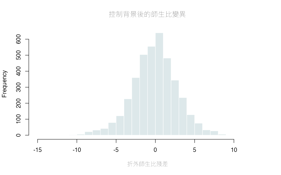
var(v_hat) 是剩餘師生比變異的診斷:若它接近零,殘差化係數便缺少可供估計的橫斷面比較。本例的正值表示演算法仍留下變異,尚不能據此判定因果重疊或不同學校具有可比的處置條件。
old_par <- par(family = plot_family)
plot(
  v_hat, u_hat,
  pch = 16, cex = 0.45, col = grDevices::adjustcolor("#173B57", 0.25),
  xlab = "交叉配適後的師生比殘差",
  ylab = "交叉配適後的測驗分數殘差",
  main = "加州學校:DML 式殘差對殘差迴歸"
)
abline(a = 0, b = theta_dml, col = "#A34045", lwd = 2)
par(old_par)
用已知真值確認殘差化公式#
下列合成資料把真實係數固定為 0.6,用來確認 Frisch–Waugh 殘差化公式與程式方向。它只是一個程式核對單元,不進入加州學校的實證結論。
set.seed(1516)
n_unit <- 5000L
X_unit <- matrix(rnorm(n_unit * 3L), ncol = 3L)
v_unit <- rnorm(n_unit)
eps_unit <- rnorm(n_unit)
D_unit <- 0.8 * X_unit[, 1] - 0.5 * X_unit[, 2] + v_unit
theta_true <- 0.6
Y_unit <- theta_true * D_unit +
  0.4 * X_unit[, 1] + 0.7 * X_unit[, 3] + eps_unit

u_unit <- residuals(lm(Y_unit ~ X_unit))
v_unit_hat <- residuals(lm(D_unit ~ X_unit))
theta_unit <- sum(v_unit_hat * u_unit) / sum(v_unit_hat^2)
stopifnot(abs(theta_unit - theta_true) < 0.05)
data.frame(truth = theta_true, partialling_estimate = theta_unit)
##   truth partialling_estimate
## 1   0.6            0.5957778
診斷圖如何幫我們下結論?#
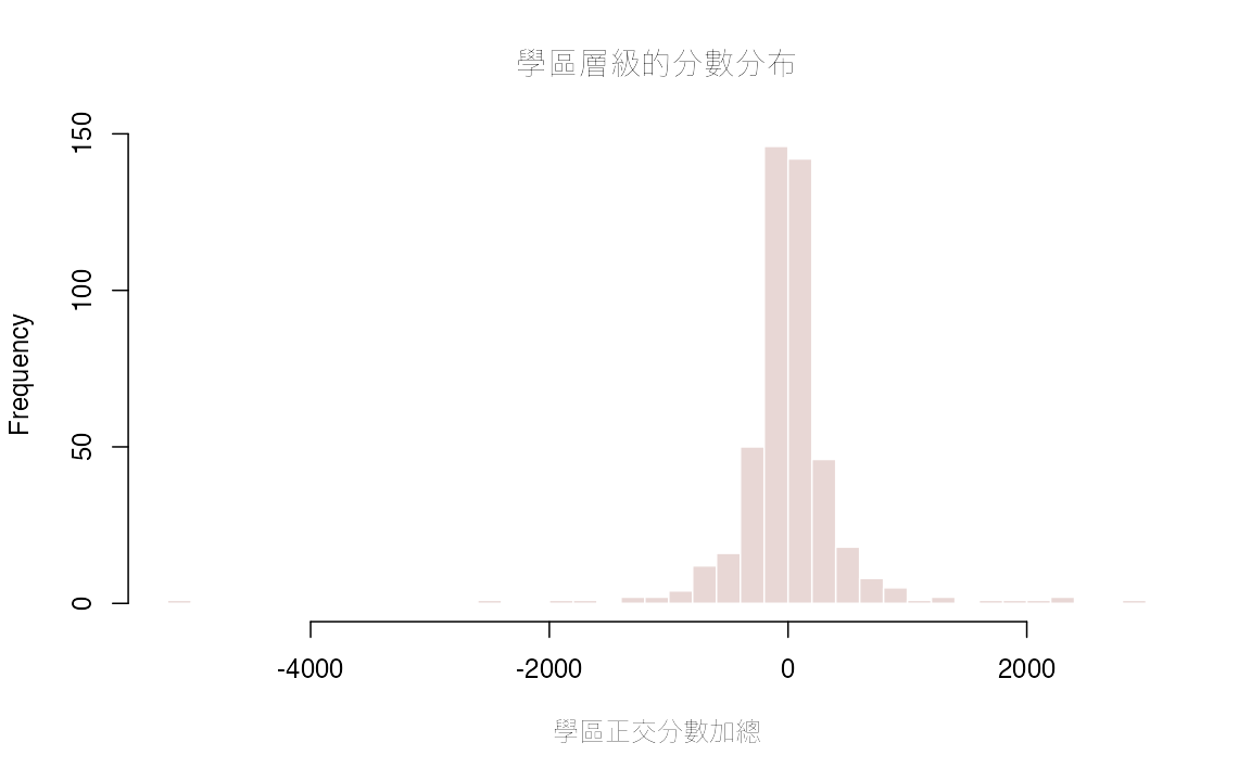
第一張圖檢查控制背景後的師生比是否仍有足夠變異,也能看出少數極端殘差是否主導斜率。第二張圖把正交分數按學區加總;若少數學區遠離其餘分布,叢聚標準誤與點估計都可能對那些學區敏感,下一步應做逐學區影響診斷。
hist(
  v_hat, breaks = 35, col = "#DDE8EA", border = "white",
  xlab = "折外師生比殘差",
  main = "控制背景後的師生比變異"
)
hist(
  as.numeric(clustered_score), breaks = 35,
  col = "#E8D7D5", border = "white",
  xlab = "學區正交分數加總",
  main = "學區層級的分數分布"
)
這份資料顯示:納入高維背景後,未調整的正向關聯大幅縮小,DML 式殘差化的點估計更接近零。適合的文字是:「在所列背景變數的部分線性投影中,str_s 每增加 1,testscore 的投影值約增加 0.075 點;學區叢聚的大樣本參考標準誤約為 0.325。這項標準誤尚未核實高維與群組漸近理論所需的全部條件,因此只作描述性參考。」
這項描述仍受資料設計限制。橫斷面檔案沒有可核實的觀察年度與處置先後;93 個控制中也可能含同步決定或處置後變數。LASSO、交叉配適與正交評分函數可以降低高維干擾函數的過度配適影響,卻不會補出時間順序、未觀察混淆或測量誤差。
若要進一步研究因果效果,下一步應先建立可信的處置時點與處置前控制集合,再檢查重疊、學區內相依及對控制字典的敏感度。統計上也可逐一移除影響較大的學區,確認點估計與大樣本參考標準誤是否由少數群組主導。
sessionInfo()
## R version 4.5.2 (2025-10-31)
## Platform: aarch64-apple-darwin20
## Running under: macOS Tahoe 26.5.1
##
## Matrix products: default
## BLAS:   /System/Library/Frameworks/Accelerate.framework/Versions/A/Frameworks/vecLib.framework/Versions/A/libBLAS.dylib
## LAPACK: /Library/Frameworks/R.framework/Versions/4.5-arm64/Resources/lib/libRlapack.dylib;  LAPACK version 3.12.1
##
## locale:
## [1] C.UTF-8/C.UTF-8/C.UTF-8/C/C.UTF-8/C.UTF-8
##
## time zone: Asia/Tokyo
## tzcode source: internal
##
## attached base packages:
## [1] stats     graphics  grDevices utils     datasets  methods   base
##
## loaded via a namespace (and not attached):
##  [1] shape_1.4.6.1       gtable_0.3.6        xfun_0.57
##  [4] ggplot2_4.0.3       collapse_2.1.7      lattice_0.22-7
##  [7] quadprog_1.5-8      vctrs_0.7.2         tools_4.5.2
## [10] Rdpack_2.6.6        generics_0.1.4      curl_7.1.0
## [13] parallel_4.5.2      sandwich_3.1-2      tibble_3.3.0
## [16] xts_0.14.2          pkgconfig_2.0.3     gbutils_0.5.1
## [19] Matrix_1.7-4        tidyverse_2.0.0     RColorBrewer_1.1-3
## [22] S7_0.2.2            lifecycle_1.0.5     compiler_4.5.2
## [25] farver_2.1.2        MatrixModels_0.5-4  maxLik_1.5-2.2
## [28] textshaping_1.0.5   codetools_0.2-20    SparseM_1.84-2
## [31] quantreg_6.1        htmltools_0.5.9     glmnet_4.1-10
## [34] Formula_1.2-5       pillar_1.11.1       MASS_7.3-65
## [37] plm_2.6-7           iterators_1.0.14    foreach_1.5.2
## [40] nlme_3.1-168        fracdiff_1.5-4      pls_2.9-0
## [43] fBasics_4052.98     tidyselect_1.2.1    bdsmatrix_1.3-7
## [46] digest_0.6.39       dplyr_1.2.1         labeling_0.4.3
## [49] splines_4.5.2       tseries_0.10-62     miscTools_0.6-30
## [52] fastmap_1.2.0       grid_4.5.2          colorspace_2.1-3
## [55] cli_3.6.5           magrittr_2.0.4      survival_3.8-3
## [58] withr_3.0.3         scales_1.4.0        forecast_9.0.2
## [61] TTR_0.24.4          rmarkdown_2.31      quantmod_0.4.29
## [64] otel_0.2.0          timeDate_4052.112   ragg_1.5.2
## [67] zoo_1.8-15          timeSeries_4052.112 fGarch_4052.93
## [70] urca_1.3-4          evaluate_1.0.5      knitr_1.51
## [73] rbibutils_2.4.1     lmtest_0.9-40       rlang_1.1.7
## [76] spatial_7.3-18      Rcpp_1.1.0          glue_1.8.0
## [79] R6_2.6.1            cvar_0.6            systemfonts_1.3.2