《財務時間序列分析》線上附錄
R10:真實股票報酬的 PCA、低秩重建與因子分析
五檔股票的報酬可否用少數幾個共同方向近似,而不失去太多橫斷面變動?把維度固定後,這個低秩表示能否延伸到較晚的月份?本附錄先用主成分分析(principal component analysis, PCA)回答這兩題,再用另一組十家公司資料示範:最大概似因子分析如何把每檔股票的標準化變異拆成共同性與個別變異。
五公司資料涵蓋 1990 年 1 月至 2008 年 12 月,共 228 個月;一列是一個月份,一欄是一家公司。十公司 Barra 資料涵蓋 1990 年 1 月至 2003 年 12 月,共 168 個月,資料排列方式相同。數值沿用原課程檔,以月報酬百分點表示,例如 4.5 代表約 4.5%;五公司檔記錄月對數報酬。資料來自原課程指向的 Ruey S. Tsay/Chicago Booth 教材檔案,隨書提供兩份固定的整理後 CSV,讓讀者可離線重做。若由上游教材檔重新整理,請保存教材版本與下載日。
PCA 與因子分析在這裡都用來描述共同變動。PCA 的跨期重建仍使用目標月份五檔股票的同月報酬來計算分數,因而不是前一期預測;旋轉後的統計因子也不會自動取得經濟名稱或因果意義。最後的合成低秩資料只檢查程式能否找回已知共同部分,不作為實證結果。
原課程程式
slides/L09_Statistical_factor_models/W2L4_hands-on_R_factors/R_script_for_factor_analysis.R
已直接使用 stats::prcomp()(原檔第 38–54 行)與 stats::factanal()(第 62–78 行);
以下保留相同的套件作法。prcomp() 代為處理中心化、標準化與奇異值分解,
factanal() 代為處理最大概似估計與旋轉;研究者仍須決定尺度、保留維度、旋轉方法、
時間切分,以及如何解讀負荷量。矩陣特徵分解、共同性與個別變異則幫助我們看清楚函數究竟算了什麼。
knitr::opts_chunk$set(
  echo = TRUE, message = FALSE, warning = FALSE,
  fig.width = 7, fig.height = 4.3
)
stopifnot(getRversion() >= "4.3.0")
set.seed(1010)
先看清楚兩組資料的觀察單位與尺度#
locate_project_file <- function(relative_path) {
  candidates <- c(
    relative_path,
    file.path("..", relative_path),
    file.path("../..", relative_path)
  )
  hit <- candidates[file.exists(candidates)]
  if (length(hit) == 0L) stop("找不到專案檔案:", relative_path)
  normalizePath(hit[1], mustWork = TRUE)
}

five_file <- locate_project_file(
  "data/processed/tsay_five_stock_monthly_returns_1990_2008.csv"
)
barra_file <- locate_project_file(
  "data/processed/tsay_barra_monthly_returns_1990_2003.csv"
)
manifest_file <- locate_project_file("data/processed/manifest.csv")

five <- read.csv(five_file, stringsAsFactors = FALSE, check.names = FALSE)
barra <- read.csv(barra_file, stringsAsFactors = FALSE, check.names = FALSE)
manifest <- read.csv(manifest_file, stringsAsFactors = FALSE)
five$month <- as.Date(five$month)
barra$month <- as.Date(barra$month)
# PCA 與跨期評量依賴時間先後,因此先明確排序再建立索引。
five <- five[order(five$month), ]
barra <- barra[order(barra$month), ]

keys <- c(
  "data/processed/tsay_five_stock_monthly_returns_1990_2008.csv",
  "data/processed/tsay_barra_monthly_returns_1990_2003.csv"
)
manifest_rows <- manifest[match(keys, manifest$file), , drop = FALSE]

stopifnot(
  nrow(five) == 228L, ncol(five) == 6L,
  nrow(barra) == 168L, ncol(barra) == 11L,
  !anyNA(five), !anyNA(barra),
  identical(unname(tools::md5sum(five_file)), manifest_rows$md5[1]),
  identical(unname(tools::md5sum(barra_file)), manifest_rows$md5[2]),
  all(diff(five$month) > 0), all(diff(barra$month) > 0)
)

rbind(
  data.frame(
    dataset = "Tsay five-stock PCA",
    first_month = min(five$month), last_month = max(five$month),
    months = nrow(five), stocks = ncol(five) - 1L,
    unit = "monthly log-return percentage points"
  ),
  data.frame(
    dataset = "Tsay Barra factor analysis",
    first_month = min(barra$month), last_month = max(barra$month),
    months = nrow(barra), stocks = ncol(barra) - 1L,
    unit = "monthly return percentage points"
  )
)
##                      dataset first_month last_month months stocks
## 1        Tsay five-stock PCA  1990-01-01 2008-12-01    228      5
## 2 Tsay Barra factor analysis  1990-01-01 2003-12-01    168     10
##                                   unit
## 1 monthly log-return percentage points
## 2     monthly return percentage points
第一張表確認兩份資料各以「月份」為觀察單位,也提醒我們不能把 4.5 誤讀成小數報酬 450%。MD5 核對只用來辨認固定資料版本;若上游教材檔更新,應重新記錄來源與轉換,而不是期待雜湊值不變。
data.frame(
  dataset = c("five-stock", "Barra ten-stock"),
  original_course_file = c("m-5clog-9008.txt", "m-barra-9003.txt"),
  source = c(
    "Ruey S. Tsay, Analysis of Financial Time Series, 3e, Example 9.2",
    "Ruey S. Tsay, Analysis of Financial Time Series, 3e, Example 9.4"
  ),
  identification_boundary = c(
    "PCA 是共同變動的描述,不識別經濟衝擊",
    "旋轉負荷量不是已命名或具因果意義的結構因子"
  )
)
##           dataset original_course_file
## 1      five-stock     m-5clog-9008.txt
## 2 Barra ten-stock     m-barra-9003.txt
##                                                             source
## 1 Ruey S. Tsay, Analysis of Financial Time Series, 3e, Example 9.2
## 2 Ruey S. Tsay, Analysis of Financial Time Series, 3e, Example 9.4
##                      identification_boundary
## 1       PCA 是共同變動的描述,不識別經濟衝擊
## 2 旋轉負荷量不是已命名或具因果意義的結構因子
套件作法:用 prcomp() 找出五檔股票的共同方向#
五家公司為 IBM、HPQ、INTC、JPM 與 BAC。先依時間固定分成 60% 估計期、20% 驗證期、20% 測試期。估計期決定中心、尺度、負荷量與維度規則;驗證期用來觀察這個規則能否延伸到較晚月份;測試期保留到最後,只評量選定維度後的低秩重建。
原課程用一行 prcomp(..., center = TRUE, scale. = TRUE) 完成估計。標準化使每檔股票先以自己的波動尺度衡量,避免高波動股票只因單位較大就支配第一主成分。緊接著的特徵分解會比較特徵值與前兩個主成分所張成的投影空間,讓讀者看見套件輸出和矩陣計算的關係。
X_five <- as.matrix(five[, -1, drop = FALSE])
storage.mode(X_five) <- "double"
n_five <- nrow(X_five)
estimate_end <- floor(0.60 * n_five)
validation_end <- floor(0.80 * n_five)
estimate_id <- seq_len(estimate_end)
validation_id <- (estimate_end + 1L):validation_end
test_id <- (validation_end + 1L):n_five

data.frame(
  sample = c("估計", "驗證", "測試"),
  first_month = five$month[c(min(estimate_id), min(validation_id), min(test_id))],
  last_month = five$month[c(max(estimate_id), max(validation_id), max(test_id))],
  months = c(length(estimate_id), length(validation_id), length(test_id))
)
##   sample first_month last_month months
## 1   估計  1990-01-01 2001-04-01    136
## 2   驗證  2001-05-01 2005-02-01     46
## 3   測試  2005-03-01 2008-12-01     46
表中的三段月份不能互換角色。特別是測試期的平均數、標準差或報酬,都不能回頭參與 prcomp() 的中心化與尺度估計。
pca_estimate <- prcomp(
  X_five[estimate_id, , drop = FALSE],
  center = TRUE,
  scale. = TRUE
)
eigenvalues <- pca_estimate$sdev^2
PVE <- eigenvalues / sum(eigenvalues)
explained <- data.frame(
  component = seq_along(PVE),
  eigenvalue = eigenvalues,
  PVE = PVE,
  cumulative_PVE = cumsum(PVE)
)
explained
##   component eigenvalue        PVE cumulative_PVE
## 1         1  2.4976099 0.49952198      0.4995220
## 2         2  1.0830169 0.21660338      0.7161254
## 3         3  0.6193526 0.12387051      0.8399959
## 4         4  0.5114440 0.10228880      0.9422847
## 5         5  0.2885766 0.05771533      1.0000000
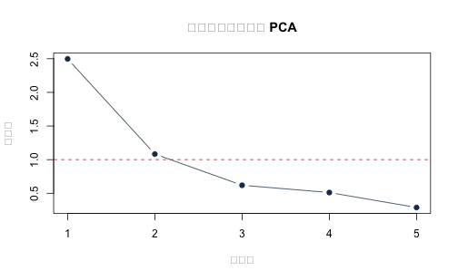
第一主成分解釋估計期約 50.0% 的標準化變異,前兩個合計約 71.6%,前三個則約 84.0%。陡坡圖與累積解釋比例都顯示:一個共同方向很重要,但只保留一個成分會漏掉相當多的橫斷面變動。
plot(
  explained$component, explained$eigenvalue,
  type = "b", pch = 19, col = "#173B57",
  xlab = "主成分", ylab = "特徵值",
  main = "五檔股票月報酬的 PCA"
)
abline(h = 1, lty = 2, col = "#A34045")
為什麼 prcomp() 與直接特徵分解會得到同一空間?#
Z_estimate <- scale(
  X_five[estimate_id, , drop = FALSE],
  center = pca_estimate$center,
  scale = pca_estimate$scale
)
eigen_direct <- eigen(cov(Z_estimate), symmetric = TRUE)
stopifnot(isTRUE(all.equal(
  unname(eigenvalues), unname(eigen_direct$values), tolerance = 1e-10
)))

projection_prcomp <- tcrossprod(pca_estimate$rotation[, 1:2, drop = FALSE])
projection_eigen <- tcrossprod(eigen_direct$vectors[, 1:2, drop = FALSE])
data.frame(
  largest_eigenvalue_difference = max(abs(eigenvalues - eigen_direct$values)),
  two_component_projection_difference =
    max(abs(projection_prcomp - projection_eigen))
)
##   largest_eigenvalue_difference two_component_projection_difference
## 1                  2.220446e-15                        6.938894e-16
兩種方法的特徵值與二維投影差異都只在浮點數誤差範圍。主成分向量乘以 $-1$ 仍代表同一條軸,因此比較時應看投影空間或重建結果,而不是把某一個負荷量的正負號當成唯一識別。
三個主成分能否重建較晚月份?#
維度選擇先寫成一條可重複的規則:取估計期累積解釋比例達 80% 的最小維度。這份資料選出三個主成分,估計期累積解釋比例約 84.0%。驗證期只用來觀察重建品質,不因結果好壞再修改 80% 門檻。
r_selected <- which(explained$cumulative_PVE >= 0.80)[1]
data.frame(
  selected_components = r_selected,
  training_cumulative_PVE = explained$cumulative_PVE[r_selected]
)
##   selected_components training_cumulative_PVE
## 1                   3               0.8399959
reconstruct_from_pca <- function(fit, newdata, r) {
  # 新月份沿用估計期中心、尺度與負荷量,避免把未來分配資訊帶回模型。
  Z <- scale(newdata, center = fit$center, scale = fit$scale)
  V <- fit$rotation[, seq_len(r), drop = FALSE]
  Z_hat <- (Z %*% V) %*% t(V)
  X_hat <- sweep(Z_hat, 2, fit$scale, "*")
  list(
    standardized_actual = Z,
    standardized_reconstructed = Z_hat,
    original_reconstructed = sweep(X_hat, 2, fit$center, "+")
  )
}

reconstruction_score <- function(actual, reconstruction) {
  Z <- reconstruction$standardized_actual
  Z_hat <- reconstruction$standardized_reconstructed
  c(
    original_scale_MSE = mean(
      (actual - reconstruction$original_reconstructed)^2
    ),
    standardized_MSE = mean((Z - Z_hat)^2),
    standardized_fraction_reconstructed =
      1 - sum((Z - Z_hat)^2) / sum(Z^2)
  )
}

validation_reconstruction <- reconstruct_from_pca(
  pca_estimate, X_five[validation_id, , drop = FALSE], r_selected
)
validation_score <- reconstruction_score(
  X_five[validation_id, , drop = FALSE], validation_reconstruction
)
validation_score
##                  original_scale_MSE                    standardized_MSE
##                          15.6180780                           0.1232204
## standardized_fraction_reconstructed
##                           0.8640172
評分沿用估計期的中心與尺度,在標準化空間比較實現值 \(Z\) 與重建值 \(\widehat Z\)。這樣估計期的 80% 選維規則與較晚月份的重建比例使用同一尺度;原始百分點 MSE 另列一欄,不能和解釋變異比例混為一談。三成分在驗證期重建約 86.4% 的標準化變動,顯示估計期找到的低維空間並未在下一段月份立即失效。這是同月重建品質,不是報酬方向的預測準確率。
選定三個成分後,以估計期加驗證期重新估計一次 PCA,再只在最後測試期評量。重新估計可利用較多歷史月份更新中心、尺度與負荷量,但不改變已選好的維度。
development_id <- c(estimate_id, validation_id)
pca_development <- prcomp(
  X_five[development_id, , drop = FALSE],
  center = TRUE, scale. = TRUE
)
test_reconstruction <- reconstruct_from_pca(
  pca_development, X_five[test_id, , drop = FALSE], r_selected
)
test_score <- reconstruction_score(
  X_five[test_id, , drop = FALSE], test_reconstruction
)
data.frame(
  selected_components = r_selected,
  validation_original_scale_MSE =
    unname(validation_score["original_scale_MSE"]),
  test_original_scale_MSE = unname(test_score["original_scale_MSE"]),
  validation_standardized_fraction =
    unname(validation_score["standardized_fraction_reconstructed"]),
  test_standardized_fraction =
    unname(test_score["standardized_fraction_reconstructed"])
)
##   selected_components validation_original_scale_MSE test_original_scale_MSE
## 1                   3                      15.61808                 12.4048
##   validation_standardized_fraction test_standardized_fraction
## 1                        0.8640172                  0.8609249
測試期原始百分點 MSE 約為 12.40,在與選維規則一致的標準化尺度上,重建比例約為 86.1%。請再次注意,程式先看到目標月份五檔股票的同月報酬,才計算該月主成分分數與重建;它回答「少數共同方向能保留多少同月資訊」,不是以前一期資訊預測下一期報酬。
套件作法:用 factanal() 分解共同性與個別變異#
第二個問題改用 Barra 十公司資料:三個潛在因子可以解釋每檔股票多少標準化變異,剩下多少屬於個別變異?factanal() 的最大概似因子分析正好提供這個分解。以下使用完整的 1990–2003 年樣本估計三因子並作 varimax 旋轉;這一節是全樣本描述,沒有訓練/測試切分,也不評估保留期績效。
原課程直接使用這個高階函數。它代為處理最大概似最佳化、三因子負荷量與 varimax 旋轉;研究者仍須事先決定因子數、資料尺度與旋轉方式,並檢查解是否容易受到樣本或規格影響。fa_three$loadings 是旋轉後負荷量,fa_three$uniquenesses 是個別變異,兩者合起來提供下表的共同性分解。factanal() 預設不讓個別變異低於 0.005;若估計值剛好停在這個下界,就屬於 Heywood/近 Heywood 警訊,不能把共同性與名目配適檢定照一般內點解解讀。
X_barra <- as.matrix(barra[, -1, drop = FALSE])
storage.mode(X_barra) <- "double"
fa_three <- factanal(
  X_barra,
  factors = 3,
  rotation = "varimax",
  scores = "regression",
  lower = 0.005
)
loadings_matrix <- unclass(fa_three$loadings)

factor_summary <- data.frame(
  stock = rownames(loadings_matrix),
  communality = rowSums(loadings_matrix^2),
  uniqueness = fa_three$uniquenesses,
  at_lower_bound = abs(fa_three$uniquenesses - 0.005) < 1e-7
)
round(loadings_matrix, 3)
##      Factor1 Factor2 Factor3
## AGE    0.678   0.217   0.121
## C      0.740   0.258   0.213
## MWD    0.818   0.356   0.062
## MER    0.819   0.328   0.070
## DELL   0.103   0.547   0.019
## HPQ    0.231   0.771   0.080
## IBM    0.200   0.514   0.239
## AA     0.195   0.545   0.499
## CAT    0.199   0.137   0.968
## PG     0.331  -0.018   0.070
factor_summary
##      stock communality uniqueness at_lower_bound
## AGE    AGE   0.5213440  0.4786595          FALSE
## C        C   0.6590180  0.3409821          FALSE
## MWD    MWD   0.7989332  0.2010671          FALSE
## MER    MER   0.7836121  0.2163876          FALSE
## DELL  DELL   0.3098410  0.6901433          FALSE
## HPQ    HPQ   0.6547619  0.3452369          FALSE
## IBM    IBM   0.3616132  0.6383908          FALSE
## AA      AA   0.5835561  0.4164444          FALSE
## CAT    CAT   0.9950005  0.0050000           TRUE
## PG      PG   0.1150995  0.8848912          FALSE
data.frame(
  nominal_likelihood_ratio_p = fa_three$PVAL,
  minimum_uniqueness = min(fa_three$uniquenesses),
  boundary_stocks = paste(
    names(fa_three$uniquenesses)[factor_summary$at_lower_bound],
    collapse = ", "
  )
)
##           nominal_likelihood_ratio_p minimum_uniqueness boundary_stocks
## objective                 0.08890732              0.005             CAT
PG 的共同性約為 0.12,表示大部分變異仍留在個別成分。CAT 看似接近 1,卻是因為個別變異剛好停在 0.005 下界;合宜的說法不是「三因子幾乎完整解釋 CAT」,而是「CAT 產生邊界解,普通三因子規格可能不足或資料不符合一般最大概似條件」。輸出的 0.089 只能稱為在獨立同分配多變量常態、內點解參考下的名目 $p$ 值;邊界解、厚尾與時間相依都會使這個參考分配變得脆弱。
接著同時改變因子數與個別變異下界。若 CAT 的個別變異總是貼著人為設定的下界,便表示「CAT 共同性接近 1」不是穩健的實證結論。這張表是規格敏感度檢查,不是正式的因子數選擇檢定。
factor_sensitivity <- do.call(rbind, lapply(2:4, function(k) {
  do.call(rbind, lapply(c(0.001, 0.005, 0.010), function(lower_bound) {
    fit <- factanal(
      X_barra, factors = k, rotation = "varimax",
      lower = lower_bound
    )
    data.frame(
      因子數 = k,
      個別變異下界 = lower_bound,
      CAT個別變異 = unname(fit$uniquenesses["CAT"]),
      CAT共同性 = 1 - unname(fit$uniquenesses["CAT"]),
      CAT是否貼住下界 =
        abs(unname(fit$uniquenesses["CAT"]) - lower_bound) < 1e-7,
      名目配適p值 = fit$PVAL,
      check.names = FALSE
    )
  }))
}))
factor_sensitivity
##             因子數 個別變異下界 CAT個別變異 CAT共同性 CAT是否貼住下界
## objective        2        0.001   0.5969104 0.4030896           FALSE
## objective1       2        0.005   0.5969104 0.4030896           FALSE
## objective2       2        0.010   0.5969104 0.4030896           FALSE
## objective3       3        0.001   0.0010000 0.9990000            TRUE
## objective11      3        0.005   0.0050000 0.9950000            TRUE
## objective21      3        0.010   0.0100000 0.9900000            TRUE
## objective4       4        0.001   0.0010000 0.9990000            TRUE
## objective12      4        0.005   0.0050000 0.9950000            TRUE
## objective22      4        0.010   0.0100000 0.9900000            TRUE
##              名目配適p值
## objective   2.463529e-06
## objective1  2.463529e-06
## objective2  2.463529e-06
## objective3  8.918147e-02
## objective11 8.890732e-02
## objective21 8.855654e-02
## objective4  2.827231e-01
## objective12 2.815853e-01
## objective22 2.801487e-01
兩因子時 CAT 沒有碰到下界,但名目配適檢定明顯較差;三、四因子時 CAT 又隨設定的下界移動。這說明因子數增加改善整體近似的同時,也暴露 CAT 的邊界問題。因而後面的負荷量圖只用來探索共同變動圖樣,不把 CAT 的共同性當成精確估計,也不宣稱三因子已通過正式模型檢定。
decomposition_gap <- max(abs(
  factor_summary$communality + factor_summary$uniqueness - 1
))

stopifnot(
  inherits(pca_estimate, "prcomp"),
  inherits(fa_three, "factanal"),
  decomposition_gap < 5e-4
)

data.frame(
  分析工作 = c("主成分分析", "最大概似因子分析"),
  原課程套件寫法 = c(
    "stats::prcomp(center = TRUE, scale. = TRUE)",
    "stats::factanal(factors = 3, rotation = 'varimax')"
  ),
  本頁物件 = c("pca_estimate", "fa_three"),
  核對內容 = c(
    "特徵值與兩主成分投影,對照直接使用 eigen() 的結果",
    "旋轉後負荷量、共同性、個別變異與配適統計量"
  ),
  數值核對 = c(
    sprintf(
      "最大特徵值差距 = %.3e",
      max(abs(eigenvalues - eigen_direct$values))
    ),
    sprintf("最大 |共同性 + 個別變異 - 1| = %.3e", decomposition_gap)
  ),
  check.names = FALSE
)
##           分析工作                                     原課程套件寫法
## 1       主成分分析        stats::prcomp(center = TRUE, scale. = TRUE)
## 2 最大概似因子分析 stats::factanal(factors = 3, rotation = 'varimax')
##       本頁物件                                          核對內容
## 1 pca_estimate 特徵值與兩主成分投影,對照直接使用 eigen() 的結果
## 2     fa_three        旋轉後負荷量、共同性、個別變異與配適統計量
##                                   數值核對
## 1               最大特徵值差距 = 2.220e-15
## 2 最大 |共同性 + 個別變異 - 1| = 1.565e-05
barplot(
  t(abs(loadings_matrix)), beside = TRUE,
  col = c("#173B57", "#A34045", "#1D6D73"),
  names.arg = rownames(loadings_matrix),
  las = 2, ylab = "因子負荷量絕對值",
  main = "十家公司月報酬的旋轉後負荷量"
)
legend(
  "topright", paste0("因子 ", 1:3),
  fill = c("#173B57", "#A34045", "#1D6D73"), bty = "n"
)
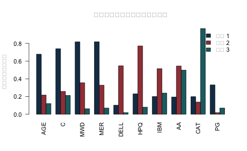
旋轉使負荷量更容易呈現群組:前兩個因子分別在部分金融與科技公司上較高,第三因子明顯集中於 CAT。這些圖樣可協助描述共同變動,但公司名稱與統計負荷量本身不足以把因子命名為特定產業、風險或結構性衝擊;命名需要額外變數與可檢驗的經濟論證。
已知真值時,兩個主成分能找回共同部分嗎?#
模擬只用於確認「保留正確共同維度可以接近真共同部分」的程式性質,不作實證結論。
set.seed(1010)
n_sim <- 600L
F_true <- matrix(rnorm(n_sim * 2L), ncol = 2L)
B_true <- rbind(
  c(0.9, 0.1), c(0.8, 0.2), c(0.7, 0.1),
  c(0.1, 0.9), c(0.2, 0.8), c(0.1, 0.7)
)
common_true <- F_true %*% t(B_true)
X_sim <- common_true + matrix(rnorm(n_sim * 6L, sd = 0.15), ncol = 6L)
pc_sim <- prcomp(X_sim, center = TRUE, scale. = FALSE)
common_hat_centered <-
  pc_sim$x[, 1:2, drop = FALSE] %*% t(pc_sim$rotation[, 1:2, drop = FALSE])
common_true_centered <- scale(common_true, center = TRUE, scale = FALSE)
common_correlation <- cor(
  as.vector(common_true_centered), as.vector(common_hat_centered)
)
stopifnot(common_correlation > 0.95)
data.frame(
  true_rank = 2L,
  retained_components = 2L,
  correlation_with_true_common_part = common_correlation
)
##   true_rank retained_components correlation_with_true_common_part
## 1         2                   2                         0.9944641
相關係數高於 0.95,說明這段程式在訊號強、維度已知的設計下能抓到共同部分。這只是程式與直覺的單元檢查;真實資料沒有可觀察的「真共同部分」,所以不能把模擬成功當成實證模型正確的證明。
從降維結果回到研究目的#
五公司資料顯示,三個主成分在較晚的測試月份仍可重建約八成以上的同月標準化變動。評分與估計期的選維規則採同一尺度;原始百分點 MSE 則另行報告。若研究目的只是壓縮資料或建立低秩共變異數近似,這是有用的起點;若目的是預測,則要另外設計只使用預測形成時已知資訊的因子分數或動態模型。
十公司因子分析則顯示,共同性在公司之間差異很大;CAT 的個別變異碰到 factanal() 下界,不能把接近 1 的共同性當成精確證據,名目配適 $p$ 值也不足以宣告三因子模型成立。旋轉讓圖樣容易閱讀,卻沒有解決邊界解、因子命名與結構識別。下一步可以比較不同因子數、旋轉方法與分段樣本,並以區塊拔靴或其他能反映時間相依的程序檢查穩定性。
重做時請保留月百分點尺度、教材版本與時間切分。若把資料先轉成小數,所有 MSE 數值會隨尺度平方改變,但解釋比例與主成分空間不應因此被重新賦予不同經濟意義。
sessionInfo()
## R version 4.5.2 (2025-10-31)
## Platform: aarch64-apple-darwin20
## Running under: macOS Tahoe 26.5.1
##
## Matrix products: default
## BLAS:   /System/Library/Frameworks/Accelerate.framework/Versions/A/Frameworks/vecLib.framework/Versions/A/libBLAS.dylib
## LAPACK: /Library/Frameworks/R.framework/Versions/4.5-arm64/Resources/lib/libRlapack.dylib;  LAPACK version 3.12.1
##
## locale:
## [1] C.UTF-8/C.UTF-8/C.UTF-8/C/C.UTF-8/C.UTF-8
##
## time zone: Asia/Tokyo
## tzcode source: internal
##
## attached base packages:
## [1] stats     graphics  grDevices utils     datasets  methods   base
##
## loaded via a namespace (and not attached):
##  [1] Matrix_1.7-4        gtable_0.3.6        dplyr_1.2.1
##  [4] compiler_4.5.2      gbutils_0.5.1       fBasics_4052.98
##  [7] tidyselect_1.2.1    Rcpp_1.1.0          cvar_0.6
## [10] parallel_4.5.2      systemfonts_1.3.2   scales_1.4.0
## [13] timeSeries_4052.112 textshaping_1.0.5   lattice_0.22-7
## [16] ggplot2_4.0.3       R6_2.6.1            generics_0.1.4
## [19] fGarch_4052.93      knitr_1.51          rbibutils_2.4.1
## [22] tibble_3.3.0        spatial_7.3-18      forecast_9.0.2
## [25] timeDate_4052.112   pillar_1.11.1       RColorBrewer_1.1-3
## [28] rlang_1.1.7         urca_1.3-4          xfun_0.57
## [31] S7_0.2.2            otel_0.2.0          cli_3.6.5
## [34] magrittr_2.0.4      Rdpack_2.6.6        grid_4.5.2
## [37] lifecycle_1.0.5     nlme_3.1-168        fracdiff_1.5-4
## [40] vctrs_0.7.2         evaluate_1.0.5      glue_1.8.0
## [43] farver_2.1.2        ragg_1.5.2          zoo_1.8-15
## [46] colorspace_2.1-3    tools_4.5.2         pkgconfig_2.0.3